Cross Validation

Brenden Ackerson, Lindsey Cook, Dominic Gallelli

An Introduction to CV

Cross Validation is a method in which we evaluate how well a model can predict values accurately. This procedure can be used to determine the best model for a data set, which is primarily used for machine learning.

Steps

Split the data into a training set and test set
Fit a model to the training set and obtain the model parameters
Apply the fitted model to the test set and obtain prediction accuracy
Repeat steps one through three
Calculate the average cross-validation prediction accuracy across all the repetitions

(Song, Tang, and Wee 2021)

How to pick the best model?

There are a many ways we can assess how well we have fit our model but typically the root mean squared error (RMSE), mean absolute error (MAE), and R-squared (\(R^2\)) are used the most. Below are formulas used to calculate each measure. RMSE calculates how far predicted values are from observed values. MAE describes the typical magnitude of the residuals. \(R^2\) describes how well the predictors explain the response variable variation, or the fraction of the variance that is explained in the model.

Evaluating the best model:

\[RMSE= \sqrt{\frac{\sum(P_i - O_i)^2}{n}}\]

\[MAE=\frac{1}{n}\sum(|y_i-\hat{y}|)\]

\[R^2=1-\frac{\sum(y_i-\hat{y})^2}{\sum(y_i-\overline{y})^2}\]

Limitations

One negative of cross-validation methods is that they are not guaranteed to pick the true model of the data distribution, even as the sample size approaches infinity. This is because when you train two different models on the same training set the one with more free parameters will model the training data better because it can over fit the data more easily. This can result in picking the wrong model due to over fitting. (Gronau and Wagenmakers 2019)

Hold Out or Validation Technique

This is the most common method of performing cross-validation (Ahmed, 2019). This method tends to use defined splits for the training and test set, like a 90/10, 80/20, etc. train/test data split. It is considered an easy, straightforward approach, but with the model only being built on a portion of the data, this model may not lead to accurate predictions because it is sensitive to what data is (or is not) chosen in the training set. This is especially problematic for small sample sizes.

k-folds Cross-Validation Technique

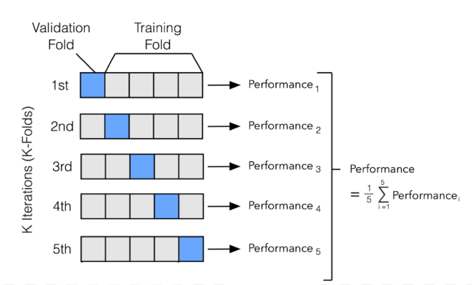
This method may be one potential answer to the limitations in the simple hold-out technique. The data is divided into k groups or splits, and then each k group becomes a test set while the other groups as a whole are the training set.

k-folds Cross-Validation Steps:

Randomly and evenly split the data set into k-folds.
Use k-1 folds of data as the training set to fit the model
With the fitted models, predict the value of the response variable in the hold out fold (kth fold)
From the response variable in the hold-out fold, calculate the prediction error

k-folds Cross-Validation Steps (contd):

Repeat steps 2-4 for k times, so each k fold is used as a hold-out
Compare the prediction performance measures to select the best model using the equation:

\[CV_(k)=\frac{1}{k}\sum_{i=1}^{k}{MSE_i}\]

(Jung2015ak?)

Figure 1

The following image visually shows the how data is split in the k-folds technique.

Figure 1: Visual Depiction of K-folds Sourced from www.i2tutorials.com for image

Repeated k-folds Cross-Validation

This methods expands on the k-folds technique (Song, Tang, and Wee 2021) by conducting multiple repetitions (n), each using a different k fold split. If 5 repeats of a 10-fold cross validation were chosen, 50 (n*k) different models would be fit and evaluated. With each repetition (n) having a slightly different data subset, the model predictors should be even more unbiased than with k-folds. One negative associated with this method is having to repeat the process numerous times, which makes this a time and labor intensive method.

Repeated k-folds Cross-Validation Steps

The process is as follows:

Randomly and evenly split the data set into k-folds.
Use k-1 folds of data as the training set to fit the model
With the fitted models, predict the value of the response variable in the hold out fold (kth fold)
From the response variable in the hold-out fold, calculate the prediction error
Repeat steps 2-4 for k times, so each k fold is used as a hold-out
Repeat steps 1-5 n times.

Leave-One-Out Cross-Validation

This method is a special case of the k-folds technique that systematically excludes each entry in the data set and fits the model with all other n-1 entries. This technique splits the data into sets of n-1 and 1, n times. For each observation, the cross-validation residual is the difference between the observation and the model predicted value. This technique has the advantages of having a less biased MSE than a single test but can be a time-consuming technique when the data set is large or the model is complex, and can thus be an expensive method. (Derryberry 2014)

Leave-One-Out Cross-Validation Steps

Split the data into a training set and testing set, using all but one observation as part of the training set.
Use the training set to build the model
Use the model to predict the response value of the one observation left out of the model
Repeat the process n times
Average the test predictions for overall model prediction values. \[CV_(n)=\frac{1}{n}\sum_{i=1}^{n}{MSE_i}\]

Optimal Number of Folds

Something to consider during the k-folds method is what is the optimal number of folds (also known as k) that the data should be divided into. In the article “Performance of Machine Learning Algorithms with Different K Values in K-fold Cross-Validation” k-validation was used on 4 different machine learning algorithms with splits of 3, 5, 7, 10, 15 and 20. They found the optimal k folds changed depending on the model being tested. (Nti, Nyarko-Boateng, and Aning 2021) Common practice uses 5 and 10 folds as these values have been shown to yield favorable test error rate estimates. (James 2013). Our paper will explore using 3, 5 and 10 k-folds, and modeling repeated k-folds of 3 and 5 repetitions on 10 folds.

Monte Carlo Cross-Validation Technique

This technique is similar to a k-fold method, but a predefined portion of the data is randomly selected to form the test set in each repetition, and the remaining portion forms the training set. The train-test process is repeated a predetermined number of times. (Wainer and Cawley 2021)

Multiple Predicting Cross-Validation

This is a variation of k-folds but instead of each fold being the validation set, it is the training set. The trained model is then evaluated on the remaining data. The average of the k-folds is then used to measure how good the model is. (Jung 2018)

Data Analysis

Hold-out validation, k-folds, repeated k-folds, leave-one-out and Monte Carlo cross-validation techniques were performed on a data set from Kaggle titled Car data.csv. This data set allowed us to model the selling price of a used car in the United Kingdom given the variables of kilometers driven, the fuel type used, the year the car was manufactured, the seller type, and transmission type. This data has 301 cars as entries. The data is detailed in the next slide.

Data Set

Variable Name	Type	Characteristic
Selling_Price	Response	Numeric
Year	Predictor	Numeric
Kms_Driven	Predictor	Numeric
Fuel_Type	Predictor	Categorical, 3 levels
Seller_Type	Predictor	Categorical, 2 levels
Transmission	Predictor	Categorical, 2 levels

Table 1: Car Data Set for Cross Validation

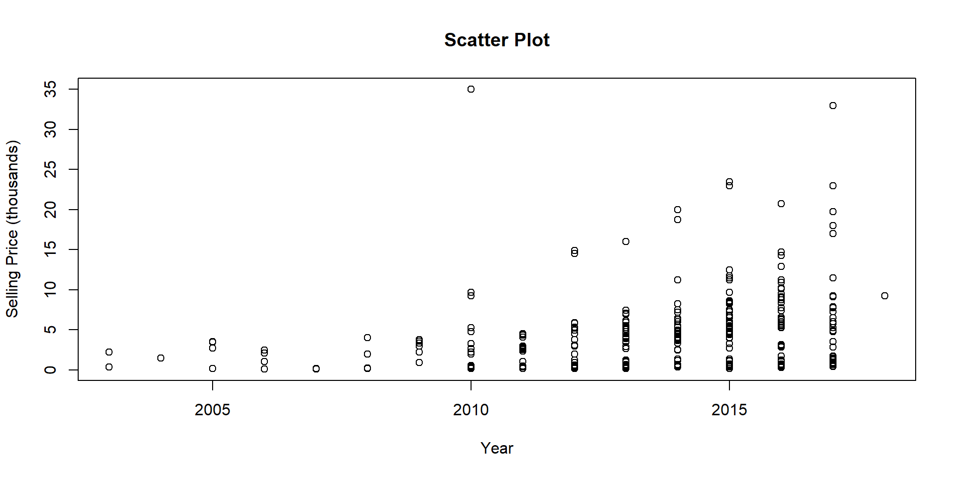
Link to Documentation for CarData data

Scatter Plot 1

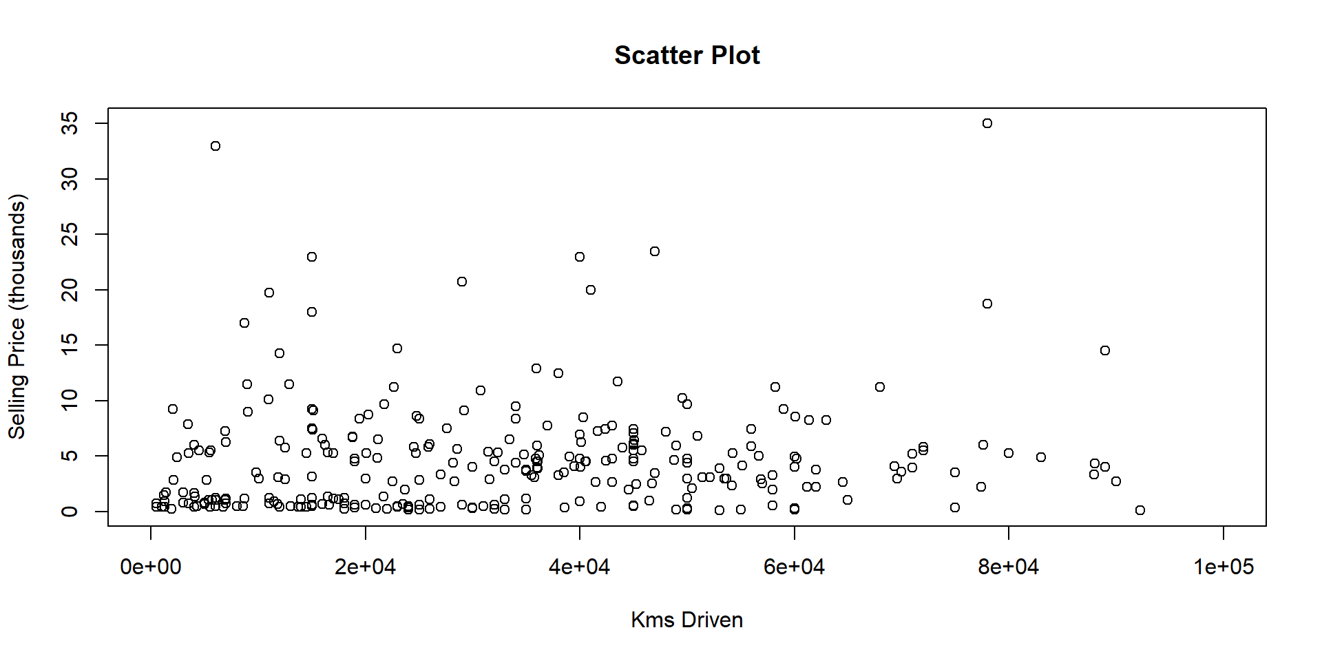
Scatter Plot 2

Linear model:

\[Selling Price=Year+KmsDriven+FuelType+SellerType+Transmission\]

This linear model was fitted using the various cross validation techniques. First the hold out method was performed using an 70/30 data split. The next technique of cross-validation was k-folds, using 3, 5, and 10 k splits. The repeated k-folds technique was then performed, using the 10 k split, repeated 3 and 5 times. Leave-one-out and Monte Carlo techniques were also ran on the model for comparisons.

Log Transformation

\[log(SellingPrice)=Year+KmsDriven+FuelType+SellerType+Transmission\]

Hold Out

library(caret)
library(ggplot2)
library(tidyverse)
library(ggfortify)
library(caTools)

set.seed(1)

car_data = read.csv("car data.csv")

# model normal linear model. 
model1 <- lm(Selling_Price ~  Kms_Driven + Fuel_Type + Seller_Type + Transmission + Year, data = car_data)
#autoplot(model1)
#summary(model1)

# Hold Out
sample <- sample.split(car_data$Year, SplitRatio = 0.7)
train  <- subset(car_data, sample == TRUE)
test   <- subset(car_data, sample == FALSE)

model_train = lm(Selling_Price ~ Kms_Driven + Fuel_Type + Seller_Type + Transmission + Year, data = train)
test_pred = predict(model_train, test)

#data.frame(R_squared = R2(test_pred, test$Selling_Price),
#           RMSE = RMSE(test_pred, test$Selling_Price),
#           MAE = MAE(test_pred, test$Selling_Price))
#  R_squared     RMSE      MAE
#  0.675032 3.066001 2.059764

k-folds Cross-Validation 10

#k-folds Cross-Validation 10
ctrl10 <- trainControl(method = "cv", number = 10)
cv_model10 <- train(Selling_Price ~ Kms_Driven + Fuel_Type + Seller_Type + Transmission + Year,
                   method = "lm",
                   data = car_data,
                   trControl = ctrl10)
cv_model10$results

  intercept     RMSE  Rsquared      MAE   RMSESD RsquaredSD     MAESD
1      TRUE 3.177328 0.6034333 2.084711 1.219663  0.1192017 0.6096877

# RMSE      Rsquared   MAE     
#v3.177328  0.6034333  2.084711

k-folds Cross-Validation 3

#k-folds Cross-Validation 3
ctrl3 <- trainControl(method = "cv", number = 3)
cv_model3 <- train(Selling_Price ~ Kms_Driven + Fuel_Type + Seller_Type + Transmission + Year,
                   method = "lm",
                   data = car_data,
                   trControl = ctrl3)
#cv_model3$results
# RMSE  Rsquared      MAE
# 3.341571 0.5671751 2.080826

k-folds Cross-Validation 5

#k-folds Cross-Validation 5
ctrl5 <- trainControl(method = "cv", number = 5)
cv_model5 <- train(Selling_Price ~ Kms_Driven + Fuel_Type + Seller_Type + Transmission + Year,
                   method = "lm",
                   data = car_data,
                   trControl = ctrl5)
# cv_model5$results
# RMSE  Rsquared      MAE
# 3.252752 0.5970045 2.088944

10-fold repeated 5

#10-fold repeated 5
ctrl10_5 <- trainControl(method = "repeatedcv", number = 10, repeats = 5)
cv_model10_5 <- train(Selling_Price ~ Kms_Driven + Fuel_Type + Seller_Type + Transmission + Year,
                   method = "lm",
                   data = car_data,
                   trControl = ctrl10_5)
#cv_model10_5$results

#RMSE      Rsquared   MAE    
#3.230983  0.6018475  2.09941

10-fold repeated 3

#10-fold repeated 3
ctrl10_3 <- trainControl(method = "repeatedcv", number = 10, repeats = 3)
cv_model10_3 <- train(Selling_Price ~ Kms_Driven + Fuel_Type + Seller_Type + Transmission + Year,
                   method = "lm",
                   data = car_data,
                   trControl = ctrl10_3 )
#cv_model10_3$results

# RMSE      Rsquared   MAE     
# 3.188268  0.6032351  2.093896

Leave-one-out Cross-Validation

#Leave-one-out Cross-Validation
ctrlLOOCV <- trainControl(method = "LOOCV")
LOO_model <- train(Selling_Price ~ Kms_Driven + Fuel_Type + Seller_Type + Transmission + Year,
                  method = "lm",
                   data = car_data,
                   trControl = ctrlLOOCV )
#LOO_model$results

# RMSE      Rsquared   MAE     
# 3.380532  0.5563956  2.089128

Monte Carlo Cross-Validation

#Monte Carlo Cross-Validation
ctrlMC <- trainControl(method = "LGOCV", number = 10)
MC_model <- train(Selling_Price ~ Kms_Driven + Fuel_Type + Seller_Type + Transmission + Year,
                    method = "lm",
                    data = car_data,
                    trControl = ctrlMC )

#MC_model$results

# RMSE      Rsquared   MAE     
# 3.375063  0.5821096  2.077517

Log Model: Hold Out

#Log Model 

model2 <- lm(log(Selling_Price) ~  Kms_Driven + Fuel_Type + Seller_Type + Transmission + Year, data = car_data)
#autoplot(model2)
#summary(model2)

# Hold Out
samplel <- sample.split(car_data$Year, SplitRatio = 0.7)
trainl  <- subset(car_data, sample == TRUE)
testl   <- subset(car_data, sample == FALSE)

model_trainl = lm(log(Selling_Price) ~ Kms_Driven + Fuel_Type + Seller_Type + Transmission + Year, data = train)
test_predl = predict(model_trainl, testl)

data.frame(R_squared = R2(test_predl, log(testl$Selling_Price)),
           RMSE = RMSE(test_predl, log(testl$Selling_Price)),
           MAE = MAE(test_predl, log(testl$Selling_Price)))

  R_squared      RMSE       MAE
1 0.8140407 0.5523885 0.4193543

#  R_squared     RMSE      MAE

k-folds Cross-Validation 10

#k-folds Cross-Validation 10
ctrl10l <- trainControl(method = "cv", number = 10)
cv_model10l <- train(log(Selling_Price) ~ Kms_Driven + Fuel_Type + Seller_Type + Transmission + Year,
                   method = "lm",
                   data = car_data,
                   trControl = ctrl10l)
cv_model10l$results

  intercept     RMSE  Rsquared       MAE    RMSESD RsquaredSD      MAESD
1      TRUE 0.552862 0.8130131 0.4126426 0.1219634 0.07759769 0.05710986

# RMSE      Rsquared   MAE

k-folds Cross-Validation 3

#k-folds Cross-Validation 3
ctrl3l <- trainControl(method = "cv", number = 3)
cv_model3l <- train(log(Selling_Price) ~ Kms_Driven + Fuel_Type + Seller_Type + Transmission + Year,
                   method = "lm",
                   data = car_data,
                   trControl = ctrl3l)
cv_model3l$results

  intercept      RMSE  Rsquared       MAE     RMSESD RsquaredSD      MAESD
1      TRUE 0.5721903 0.8042955 0.4115007 0.06903892 0.04902898 0.03076828

k-folds Cross-Validation 5

#k-folds Cross-Validation 5
ctrl5l <- trainControl(method = "cv", number = 5)
cv_model5l <- train(log(Selling_Price) ~ Kms_Driven + Fuel_Type + Seller_Type + Transmission + Year,
                   method = "lm",
                   data = car_data,
                   trControl = ctrl5l)
cv_model5l$results

  intercept      RMSE Rsquared      MAE     RMSESD RsquaredSD      MAESD
1      TRUE 0.5323999 0.825842 0.399347 0.08631279 0.06073456 0.03252152

10-fold repeated 5

#10-fold repeated 5
ctrl10_5l <- trainControl(method = "repeatedcv", number = 10, repeats = 5)
cv_model10_5l <- train(log(Selling_Price) ~ Kms_Driven + Fuel_Type + Seller_Type + Transmission + Year,
                   method = "lm",
                   data = car_data,
                   trControl = ctrl10_5l)
cv_model10_5l$results

  intercept      RMSE Rsquared       MAE    RMSESD RsquaredSD      MAESD
1      TRUE 0.5408217 0.823465 0.4045896 0.1048676 0.06773348 0.05689064

#RMSE      Rsquared   MAE

10-fold repeated 3

#10-fold repeated 3
ctrl10_3l <- trainControl(method = "repeatedcv", number = 10, repeats = 3)
cv_model10_3l <- train(log(Selling_Price) ~ Kms_Driven + Fuel_Type + Seller_Type + Transmission + Year,
                   method = "lm",
                   data = car_data,
                   trControl = ctrl10_3l )
cv_model10_3l$results

  intercept      RMSE  Rsquared       MAE   RMSESD RsquaredSD      MAESD
1      TRUE 0.5509084 0.8174797 0.4091709 0.105851  0.0670746 0.05891568

# RMSE      Rsquared   MAE

Leave-one-out Cross-Validation

#Leave-one-out Cross-Validation
ctrlLOOCVl <- trainControl(method = "LOOCV")
LOO_modell <- train(log(Selling_Price) ~ Kms_Driven + Fuel_Type + Seller_Type + Transmission + Year,
                  method = "lm",
                   data = car_data,
                   trControl = ctrlLOOCVl )
LOO_modell$results

  intercept      RMSE Rsquared       MAE
1      TRUE 0.5564873 0.807924 0.4072408

# RMSE      Rsquared   MAE

Monte Carlo Cross-Validation

#Monte Carlo Cross-Validation
ctrlMCl <- trainControl(method = "LGOCV", number = 10)
MC_modell<- train(log(Selling_Price) ~ Kms_Driven + Fuel_Type + Seller_Type + Transmission + Year,
                    method = "lm",
                    data = car_data,
                    trControl = ctrlMCl )

MC_modell$results

  intercept      RMSE  Rsquared       MAE     RMSESD RsquaredSD     MAESD
1      TRUE 0.5382496 0.8183334 0.3981915 0.06449471 0.05304317 0.0218922

Summary: Linear Model

	Monte Carlo	k-folds k=3	k-folds k=5	k-folds k=10
RMSE	3.375063	3.389747	3.35485	3.177328
Rsquared	0.5821096	0.5431807	0.5792003	0.6034333
MAE	2.077517	2.121226	2.078258	2.084711

Summary: Linear Model (contd)

	10-fold repeated 5 times	10-fold repeated 3 times	leave one out	Hold Out
RMSE	3.230983	3.188268	3.380532	3.066001
Rsquared	0.6018475	0.6032351	0.5563956	0.675032
MAE	2.09941	2.093896	2.089128	2.059764

Summary: Log Transformation

	Monte Carlo	k-folds k=3	k-folds k=5	k-folds k=10
RMSE	0.6000005	0.5597472	0.5546057	0.5547619
Rsquared	0.7844457	0.8191809	0.81445	0.8097507
MAE	0.4230068	0.4125619	0.406683	0.4080991

Summary: Log Transformation (contd)

	10-fold repeated 5 times	10-fold repeated 3 times	leave one out	Hold Out
RMSE	0.5429957	0.5415532	0.5564873	0.5544994
Rsquared	0.8180418	0.8220338	0.807924	0.8283292
MAE	0.4056521	0.4047157	0.4072408	0.400559

Conclusion

As cross-validation tends to be used in machine learning on large data, or in situations where it may be hard to gather large samples, our example allowed us to review the full data set’s performance with linear regression and then compare the performance of the cross validation techniques. We compared both a linear model and a transformed linear model and found that for the most part many of these cross validation techniques performed about the same and were able to fit accurate models. While k-folds, repeated k-folds and hold-out seemed to perform the best, most of these techniques seem sufficient to help validate a model.

References

Derryberry, DeWayne R. 2014. Basic Data Analysis for Time Series with r. John Wiley & Sons.

Gronau, Quentin F, and Eric-Jan Wagenmakers. 2019. “Limitations of Bayesian Leave-One-Out Cross-Validation for Model Selection.” Computational Brain & Behavior 2 (1): 1–11.

James, Witten, G. 2013. An Introduction to Statistical Learning: With Applications in r. Springer.

Jung, Yoonsuh. 2018. “Multiple Predicting k-Fold Cross-Validation for Model Selection.” Journal of Nonparametric Statistics 30 (1): 197–215.

Nti, Isaac Kofi, Owusu Nyarko-Boateng, and Justice Aning. 2021. “Performance of Machine Learning Algorithms with Different k Values in k-Fold Cross-Validation.” Inter. J. Info. Technol. Comp. Sci. 13: 61–71.

Song, Q Chelsea, Chen Tang, and Serena Wee. 2021. “Making Sense of Model Generalizability: A Tutorial on Cross-Validation in r and Shiny.” Advances in Methods and Practices in Psychological Science 4 (1): 2515245920947067.

Wainer, Jacques, and Gavin Cawley. 2021. “Nested Cross-Validation When Selecting Classifiers Is Overzealous for Most Practical Applications.” Expert Systems with Applications 182: 115222.